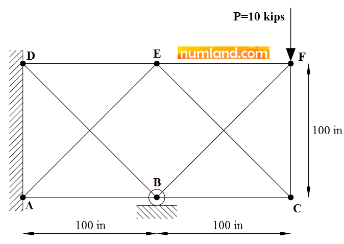
Consider the truss shown in the Figure including 9 members, which can rotate freely at the joints. The whole system is constrained at two points of A and D and a roller support of B. The members CE and BF as well as AE and BD do not intersect each other, so, there is no joint in the middle of these members. Because of manufacturing error, CF is 0.1 in shorter than the length of 100 in (99.9 in). Accordingly, there might be a pre-load in this member as well as the others related to this one. In addition, a concentrated force of 10000 lb, symbolized by P, is applied on the point F. The point of B has been pulled down 0.05 in and kept ny the support. The entire system is, also, heated in order to increase the temperature 50 oF. It causes thermal stresses in all members. This Example leads you through the Abaqus\CAE modeling process to look for the stress in CF member and reaction force in the point B. More is, the results will be compared with the reference [1]. All lengths are in inch and all members cross-sectional areas are 3.33333 in2. The members are made from steel with the modulus of elasticity of 30×106 psi and thermal expansion coefficient of ![]() .
.
There exists another type of connector named Axial, which is able to make tension in member CF, as Translator Connector was. The reason that we do not use the Translator Connector will reveal in the current Example though. Firstly, duplicate the model you created in Example 2 by using Copy Model as shown in Figure 2. Name this new model 2D truss-Axial.
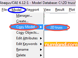
This leads to creating another model, in the Model Tree, with mentioned name. To assess sub-elements related to this model, first, click on ![]() next to the 2D truss model on which we worked in Example 2, then, as shown in Figure 3, click on
next to the 2D truss model on which we worked in Example 2, then, as shown in Figure 3, click on ![]() prior to 2D truss-Axial model in Model Tree.
prior to 2D truss-Axial model in Model Tree.

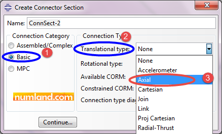
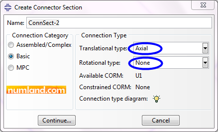
Now enter Interaction module and click on icon ![]() (Create Connector Section). As Figure 4 displays, select Axial following the sequence, which is pointed out. Finally, press Continue button.
(Create Connector Section). As Figure 4 displays, select Axial following the sequence, which is pointed out. Finally, press Continue button.
| Note 1
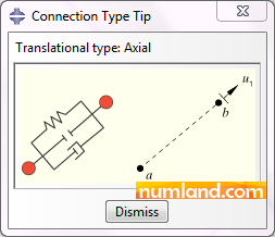
As Figure A shows, U1 next to Available CORM, same as Translator Connector tells only one translational DOF is available, although other degrees of freedom are free as None has been written beside Constrained CORM.
Click on icon
|
Same as Example 2 there is no need to define connector characteristics. So, just click on OK in Edit Connector Section window. This will create an Axial Connector Section in the model and the action we need to take after this is to replace it with the Translator Connector by use of the icon pointed out in Figure 5.
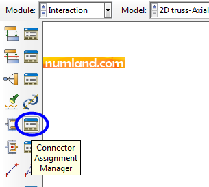
In the Connector Section Assignment Manager window, which is displayed in Figure 6, select ConnSect-1, then, click on Edit button.

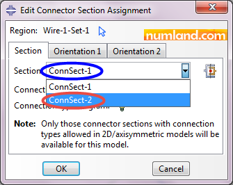
Change the Section in opened window shown in Figure 7 to ConnSect-2 which includes Axial Connector. Clicking Ok causes assigning the Axial Connector created in previous step to the points F and F’.
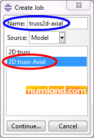
After that, enter Job module and click on icon ![]() (Create Job). As displayed in Figure 8, name this job truss2d-axial and press Continue. Note that the model of 2D truss-Axial has been selected. Next, press OK in Edit Job window and opening Job Manager, submit it to the Abaqus/CAE.
(Create Job). As displayed in Figure 8, name this job truss2d-axial and press Continue. Note that the model of 2D truss-Axial has been selected. Next, press OK in Edit Job window and opening Job Manager, submit it to the Abaqus/CAE.
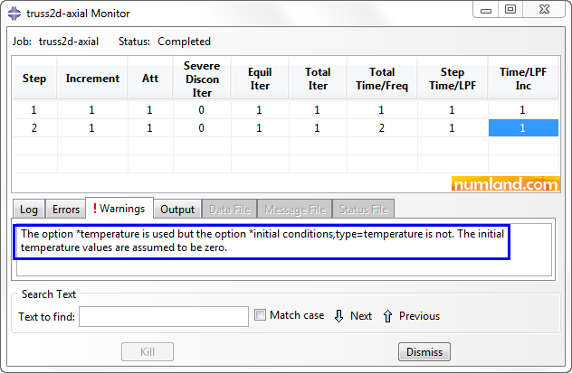
When the job has been finished, click on Monitor button, then, go to Warning tab which is shown in Figure 9. As you see, there is no pivot error which appeared when using Translator Connector. So, it seems this issue has been solved by using Axial Connector. Let’s investigate the results, then, conclude.
In order to observe the results, firstly, pick the forces in the member CF and the support B using the method mentioned among Figures 64 to 68 in Example 2. The magnitudes of these outputs are presented in Figure 10.
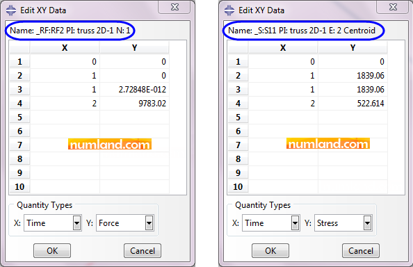
As you see, the results equal the ones obtained from the model in which Translator Connector was used. Now we evaluate displacements of the points F and F’. The procedure of doing this is explained in Figures 50 to 63 of Example 2. Figure 11 shows the changes in U1 and U2 for both points, during the time.
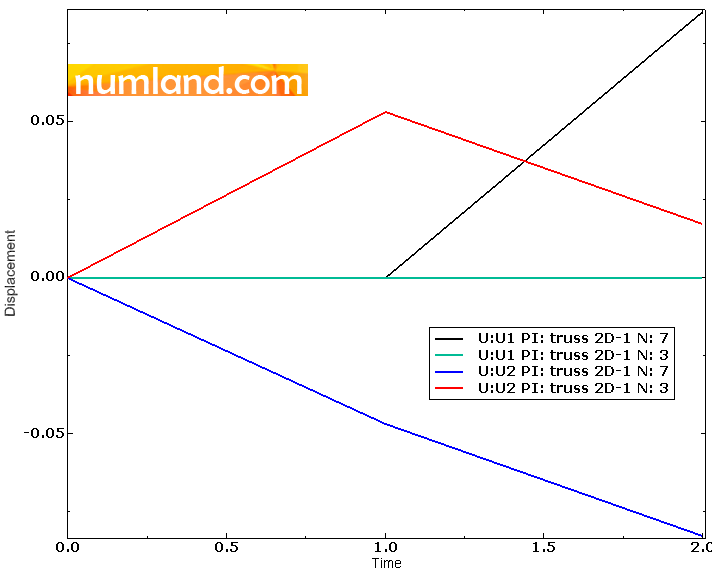
Unlike Example 2, displacements of both points in X direction are not equal. These data have been presented in Figures 12.
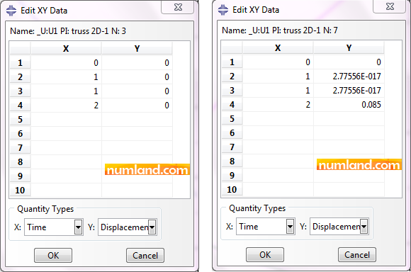
It is clear that point F’ has not moved through X direction, meanwhile F has. This means that these points did not lay on each other. To observe more, displacements of these points are presented in Figure 13.
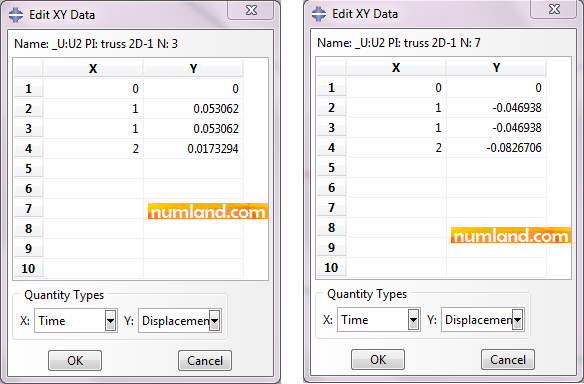
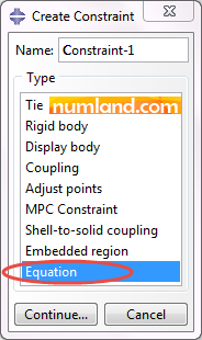
Although, in Step-1, vertical displacements of both points totally are equal to 0.1 in, which means they meet each other in this step, the points will move differently in Step-2. To deal with this issue, we need to define a constraint on U1 displacements of F and F’ by utilizing equation command. To do this, enter Interaction module and zoom on the points of F and F’. Then, click on icon ![]() (Create Constraint). In opened window select the item Equation, as shown in Figure 14.
(Create Constraint). In opened window select the item Equation, as shown in Figure 14.
As Figure 15 shows, to make an equation constraining the points, it requires to define Set, otherwise, the action would be impossible. Note as shown in the Figure, two Sets involving two points must be created.
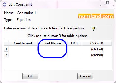
To create a Set, follow the steps below:
Tools > Set > Create
In opened window, select the items Figure 16 displays, then, Continue.
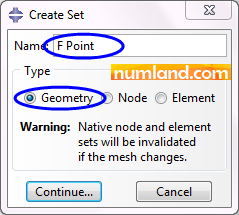
After this, select point F as specified in Figure 17 and press Done in prompt area. This makes a Set in which includes point of F.
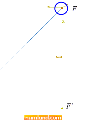
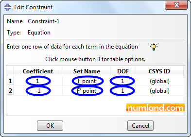
Do the same to define another Set, named F’ point, which would obviously be related to the point F’. Doing this, we can use the Equation command. Therefore, as explained above, run Create Constraint tool and select Equation item again, then, press Continue button. Figure 18 illustrates how you need to fill the items in Edit Constraint window. Finally, press OK. This makes U1 of both points remain equal.
| Note 2
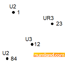
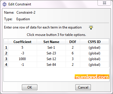
Consider a model with large number of nodes. Among them, we select 4 nodes as displayed in Figure A.
We are willing to make a relation between these degrees of freedom based on the equation below. 5×U21 – 3×UR323 + 1000×U312 – U284 = 0 To do this, insert the values presented in Figure B. Take notice we already created 4 sets, named according to the nodes number.
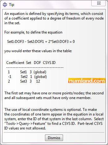
When defining equations, consider these points: The equation must be linear. Put all variables in one side of the equation [f (DOFs) =0]. DOFs of U1, U2, U3, UR1, UR2, UR3 are specified by numbers of 1, 2, 3, 4, 5, 6, respectively. For more information refer Note 11 in Example 2. The first Set can contain 1 or more points, but the other sets must only have 1 point. Otherwise you will face the error displayed below.
To find more about equation constraint, click on icon
|
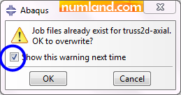
To analyze the model with new conditions, enter Job module and clicking on icon ![]() (Job Manager), submit the job named truss2d-axial again. If you saw a message involving existence of another job with the same name, disable the check box as Figure 19 shows and press OK.
(Job Manager), submit the job named truss2d-axial again. If you saw a message involving existence of another job with the same name, disable the check box as Figure 19 shows and press OK.
By the time the job has completed, check if there is any warning except initial temperature warning. Click on Results button, then, to enter Visualization module. After observing the stresses and deformed shape, evaluate forces in member CF and support B. Their magnitudes have been presented in Figure 20.
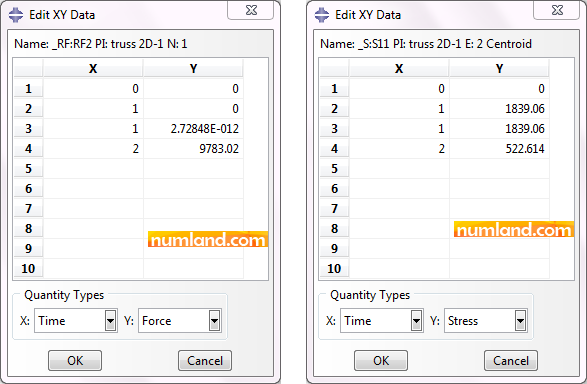
Comparing the results earned when using Translator Connector reveals these outputs are exactly equal. Now, check displacements of points F and F’ in both directions of X and Y. The results have been presented in Figures 21 and 22.
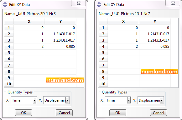
As seen, U1 displacements in Step-2 are equal. This shows the Equation constraint worked correctly.
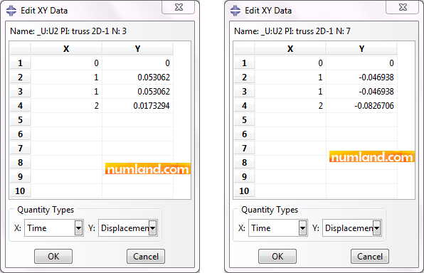
Ensure whether distance of 0.1 in between the points became 0 in Step-1. Moreover, calculate the movements of both nodes, in Step-2 as they must be equal.
Conclusion:
Despite correct answers given by using Translator Connector, we changed the connector type to the Axial so that there were warnings of zero pivot for 6th DOFs in Example 2. However, this caused a new problem with matching the points F and F’. To deal with this issue, we defined an Equation constraint. Doing this led to the validate answers without any zero pivot warnings. According all of these, being conscious about the warnings and eliminating them, during analyzes is significant, because neglecting them causes various problems that we discuss in future.
Exercise:
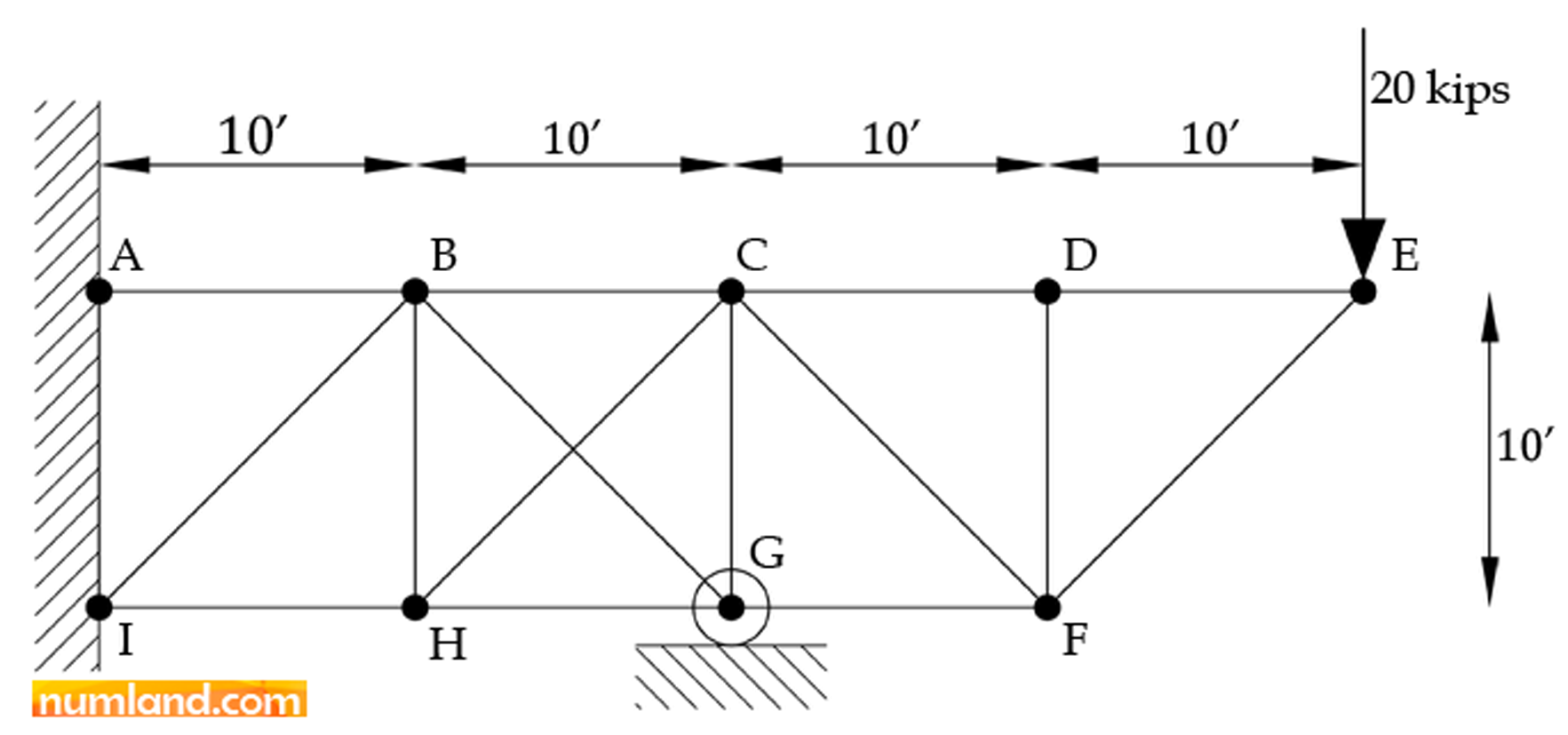
Consider the planar truss shown in Figure 23 [2]. It is made of 12 pin-jointed members. The members BG and CH do not intersect each other. Points A and I are attached to a wall. This means these points are constrained in all degrees of freedom. The joint G is a support being able to move in X direction. A force of 20 kips is applied on the point E. The point B has been pulled down 0.3 in and kept there. In this problem, we are looking for reaction force in support G. All length are given in foot. The material of all members is steel with Young’s Modulus of 30×106 psi. In addition, 2 in2 is considered as their cross-sectional area. Note that convert the lengths to inch, firstly.
Answer: RG=21000 lbs
References:
[1] Timoshenko, S. P. and Young, D. H. “Theory of Structures,” end Ed., McGraw-Hill, New York, 1965, pp. 313-315.
[2] Timoshenko, S. P. and Young, D. H. “Theory of Structures,” end Ed., McGraw-Hill, New York, 1965, pp. 309.


Be the First to Comment!